Pre-symplectic formalism and double differential forms

Many quantization procedures start from some kind of canonical formalism. A covariant canonical formalism on a group manifold has been developed in refs. [89,90]. A covariant symplectic approach to geometric field theories proposed in ref. [91] can be adapted very naturally to the theories described in the present notes and we shall follow many of its ideas, that will play an important role in the following. The symplectic structure of the phase space is the starting point of geometric quantization [67,68]. Though we have no reasonable hope to carry out the whole quantization of the classical theories we are considering, the general concepts given in the present Section may suggest some useful ideas.

It is useful to start from the analogy with a mechanical system with $d$ degrees of freedom [92,93,94]. The phase space $\Gamma$ can be interpeted as the space of motions, namely the space of the solutions of the equations of motion or of the corresponding initial conditions at a given time $t$. We indicate by $q^{\chi}$, $\chi = 1,\ldots, d$ a local system of Lagrangian coordinates, by $\dot q^{\chi}$ the corresponding velocities and we define, as usual, the canonical momenta

$$p_{\chi}(t) = \frac{\partial L}{\partial \dot q^{\chi}},$$ (4.73)

where $L(q^{\chi}, \dot q^{\chi})$ is the Lagrange function. The (closed, nondegenerate) symplectic form is given by

$$\Omega(t) = \hat d q^{\chi}(t) \wedge \hat d p_{\chi}(t), \qquad \hat d \Omega(t) = 0.$$ (4.74)

We use the symbol $\hat d$ to denote the exterior derivative of differential forms defined on $\Gamma$, in order to avoid confusion with the exterior derivative of differential forms defined on $\mathcal{S}_n$, that we continue to indicate by $d$. We also introduce the notation $\hat i(X)$ and $\hat L(X)$ for the inner product and the Lie derivative acting on the differential forms in $\Gamma$. For the exterior product, we use in both cases the symbol $\wedge$.

In the following it is useful to consider double differential forms, a concept treated with some detail in ref. [95]. A $(u, v)$-double form defined, for instance, on $\Gamma \times \mathcal{S}_n$ is given, at a given point of this manifold, by a multilinear form depending (antisymmetrically) on $u$ vectors of the tangent space of $\Gamma$ and $v$ vectors of the tangent space of $\mathcal{S}_n$. The manifold $\mathcal{S}_n$ can be replaced by the manifold that describes the geometry in other theories, for instance the spacetime $\mathcal{M}$ or, in the simple mechanical system we are now considering, the time axis $\mathbf{R}$.

The time evolution of the system is described by a one-parameter group of diffeomorphisms of $\Gamma$ generated by a vector field $X$. The dynamical variables are functions defined on $\Gamma \times \mathbf{R}$, that we can also consider as $(0,0)$-double differential forms. Their time derivative is given by

$$\frac{d}{dt} f = \dot f = X f = \hat i(X) \hat d f$$ (4.75)

and the canonical equations of motion can be written in the form

$$\hat i(X) \Omega = \hat d H,$$ (4.76)

where $H(q^{\chi}, p_{\chi})$ is the Hamiltonian function. It follows that

$$\frac{d}{d t} \Omega = \hat L(X)\Omega = \hat d \hat i(X) \Omega = \hat d \hat d H = 0,$$ (4.77)

namely the symplectic form $\Omega$ does not depend on time. This is the property that justifies its definition.

We can consider $\Omega$ as a double $(2, 0)$-form on the manifold $\Gamma \times \mathbf{R}$. More explicitly, it is at the same time a 2-form on $\Gamma$ and a 0-form (namely a function) on $\mathbf{R}$. The fact that it does not depend on $t$ can be written as $d \Omega = 0$, while $\hat d \Omega = 0$ means that, for any value of $t$, it is a closed form on $\Gamma$.

If we consider a field theory, the space $\Gamma$ is infinite-dimensional and the mathematics of differential forms [27] becomes rather delicate and also ambiguous, because one has to choose a norm, or at least a topology, in the tangent spaces. We shall not enter into these details and our proposal is admittedly deprived of any mathematical rigour. We hope that, if necessary, it will be possible to transform it into a mathematically acceptable treatment.

Following the analogy with a mechanical system we treat the quantities $\omega^{\alpha}$ and $\Psi^U$ as ``Lagrangian coordinates'' and the quantities $F_{\alpha \beta}^{\gamma}$ and $A_{\alpha} \Psi^U$ as the ``velocities''. A comparison between the normal field equations written in the form (4.29), (4.31) and eq. (4.73) suggests that the forms $\sigma_{\alpha}$ and $\pi_a$ should be considers as the ``canonical momenta'' of the theory.

A natural generalization of eq. (4.74) is

$$\Omega(\Sigma) = \int_{\Sigma} \Omega, \qquad \Omega = \hat ... ...ge \hat d \sigma_{\alpha} + \hat d \Psi^U \wedge \hat d \pi_U.$$ (4.78)

Under the integral sign, we have the $(2,3)$-double form $\Omega$, that we call the symplectic double form and represents, in some sense, a ``density'' of symplectic form. The 3-dimensional submanifold $\Sigma$ of $\mathcal{S}_n$ should be chosen with the same criteria used in Section 4.1 to define the global conserved quantities, for instance the electric charge, starting from the corresponding closed 3-forms that describe their ``densities''.

The choice of $\Sigma$ is a difficult problem, but fortunately we can prove that, as a consequence of the field equations, we have $d \Omega = 0$. As in the mechanical case, this is the crucial property of $\Omega$. It follows that $\Omega(\Sigma)$ is not affected by deformations of $\Sigma$ that modify only a compact subset and not its boundary $\partial \Sigma$. However, $\Sigma$ should extend to infinity and problems of convergence may arise. Moreover, $\Omega(\Sigma)$ could depend on the asymptotic behavior of $\Sigma$.

It has been remarked, in the framework of quantum field theory [96,97], that globally defined quantities are not really observable and that a field theory should be described in terms of local algebras of observables concerning compact regions of spacetime. Perhaps the form $\Omega(\Sigma)$ with sufficiently large but compact $\Sigma$ could be sufficient for the construction, by means of some quantization procedure, a local algebra of observables. A further development of this idea is completely outside the purposes of the present notes. In the following we do not specify the choice of $\Sigma$, since many local results can be obtained by considering the symplectic double form $\Omega$, without any reference to the symplectic form $\Omega(\Sigma)$.

The infinitesimal variations indicated by $\delta$ in the preceding Sections can be described by an infinitesimal vector field $X$ defined on $\Gamma$. If $f$ is a dynamical variable, described as a $(0,v)$-double form, its infinitesiamal variation previously indicated by $\delta f$, in the present Section should be indicated by $X f = \hat i(X) \hat d f$.

The 3-form $\theta$ defined by eq. (4.39) depends on a vector field $X$ that describes the variations indicated by the symbol $\delta$ and it is more correctly interpreted as a (1, 3)double form defined by

$$\theta = \hat d \Psi^U \wedge \pi_U + \hat d \omega^{\alpha} \wedge \sigma_{\alpha}$$ (4.79)

and eq. (4.40) gives

$$\hat i(X) d \theta = \hat i(X) \hat d \lambda.$$ (4.80)

Since $X$ is arbitrary, we obtain the important relation between $(1, 4)$-double forms

$$d \theta = \hat d \lambda,$$ (4.81)

that can be considered asd a formulation of Noether's theorem in terms of double forms. In conclusion, we have

$$\Omega = - \hat d \theta, \qquad d \Omega = - d \hat d \theta = - \hat d \hat d \lambda = 0,$$ (4.82)

as it was announced above. We also have

$$\Omega(\Sigma) = - \hat d \theta(\Sigma), \qquad \theta(\Sigma) = \int_{\Sigma} \theta$$ (4.83)

and we see that, in the circumstances we are considering, the symplectic form $\Omega(\Sigma)$, besides being a closed form, is also exact.

Many interesting theories are described by a degenerate Lagrangian and one can eliminate (locally) the ``velocities'' $F_{\alpha \beta}^{\gamma}$, $A_{\alpha} \Psi^U$ from the the normal equations (4.29) and (4.31), obtaining primary Lagrangian constraints that involve only the ``Lagrangian coordinates'' $\omega^{\alpha}$, $\Psi^U$ and the ``canonical momenta'' $\sigma_{\alpha}$ and $\pi_U$. In some cases, from the other field equations one also obtains secondary constraints. As a consequence, the states of the system are described by the points of the submanifold $\Gamma' \subset \Gamma$ defined by all the constraint equations. A more detailed dicussion of primary and secondary constraints can be found, for instance, in ref. [98]. It may be useful to remark that the submanifold $\Gamma'$ is not necessarily defined by a set of global constraint equations. It may be necessary to use different constraint equations in a neighborhoods of differnt points of $\Gamma'$.

The symplectic formalism allows a treatment of the constraints considerably simpler than the better known approach based on the Poisson and Dirac brackets [98]. If the restriction $\Omega'(\Sigma)$ of the form $\Omega(\Sigma)$ to the submanifold $\Gamma'$ is nondegenerate, $\Gamma'$ is a symplectic manifold to be identified with the phase space of the system. The corresponding Poisson brackets (different from the Poisson brackets of $\Gamma$) are called the Dirac brackets.

However, in the most interesting cases the 2-form $\Omega'(\Sigma)$ is degenerate. In this case, the space $\Gamma'$ is not a symplectic space, but a pre-symplectic space and there are vector fields $X$ on $\Gamma'$ that satisfy the condition

$$\hat i(X)\Omega'(\Sigma) = 0.$$ (4.84)

These vector fields are interpreted as the generators of gauge transformations. As a consequence of the property

$$\hat d \Omega'(\Sigma) = 0,$$ (4.85)

they define an integrable distribution of subspaces in the tangent spaces of $\Gamma'$ and one can apply Frobenius' theorem, as we have done in Section 2.3 (if there is a version of this theorem valid in the infinite-dimensional manifolds we are considering!). If the set $\Gamma''$ of the leaves has a manifold structure, one can define on it a symplectic (nondegenerate) form $\Omega''(\Sigma)$ and one obtains in this way the true phase space of the theory.

Alternatively (under suitable conditions), one can introduce, besides the Lagrangian constraints, other gauge fixing constraints that define a submanifold $\Gamma'' \subset \Gamma' \subset \Gamma$ that itersects all the leaves of $\Gamma'$ at only one point and is clearly equivalent to the set of the leaves introduced above. In this case, one can identify $\Omega''(\Sigma)$ with the restriction of $\Omega(\Sigma)$ to $\Gamma''$. We can also consider the restriction $\theta''(\Sigma)$ of the 1-form $\theta(\Sigma)$ to $\Gamma''$ and we have

$$\Omega''(\Sigma) = - \hat d \theta''(\Sigma),$$ (4.86)

namely $\Omega''(\Sigma)$ is exact. It is not necessary to assume that $\Gamma''$ is defined globally by a set of constraint equations.

However, it is not always possible to find a submanifold $\Gamma''$ with the required properties, as one can see from simple finite-dimensional examples. Then the closed form $\Omega''(\Sigma)$ does not need to be exact and may have nontrivial topological (cohomological) properties that can give rise to obstructions to the quantization procedure [67,68] unless the Planck constant $\hbar$ takes some special values, as we have shortly discussed in Section 2.4. It is for this reason that we try to give some attention to the topological properties of the phase space.

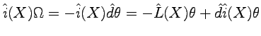
We have already remarked in Section 2.5 that the theories we are considering have gauge transformations corresponding to the diffeomorphisms of $\mathcal{S}_n$. If the vector field $B$ in $\mathcal{S}_n$ generates infinitesimal diffeomorphisms of this manifold, the vector field $X$ on $\Gamma$ that generates the corresponding gauge transformations is defined by

$$X f = \hat i(X) \hat d f = \hat L(X) f = L(B) f,$$ (4.87)

where $f$ is an arbitrary dynamical variable, namely a $(0,v)$-double form. Since the Lie derivatives are derivations of the algebra of the differential forms, this formula can be extended to an arbitrary $(u, v)$-double form $f$, namely we have in general

$$\hat L(X) f = L(B) f.$$ (4.88)

If there are Lagrangian constraints, the vector field $X$ is tangent to $\Gamma'$ and it can be considered as a vector field on this submanifold.

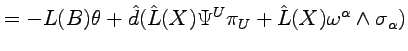
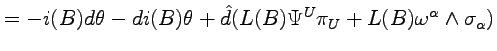
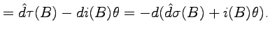
By means of the formulas given above and eq. (4.43) and (4.51), we can write

$$\hat i(X) \Omega = - \hat i(X) \hat d \theta = - \hat L(X) \theta + \hat d \hat i(X) \theta$$

$$= - L(B) \theta + \hat d (\hat L(X) \Psi^U \pi_U + \hat L(X) \omega^{\alpha} \wedge \sigma_{\alpha})$$

$$= - i(B) d \theta - d i(B) \theta + \hat d (L(B) \Psi^U \pi_U + L(B) \omega^{\alpha} \wedge \sigma_{\alpha})$$

$$= \hat d \tau(B) - d i(B) \theta = - d (\hat d \sigma(B) + i(B) \theta).$$ (4.89)

It follows that

$$\hat i(X) \Omega(\Sigma) = - \int_{\partial \Sigma} (\hat d \sigma(B) + i(B) \hat \theta)$$ (4.90)

and, if $B$ has a compact support that does not intersect the boundary $\partial \Sigma$, this expression vanishes as it is expected if $X$ generates a gauge transformation.

If $X$ generates a symmetry transformation of the kind (2.11), all the quantities that have only contracted indices are invariant and in particular we have

$$\hat L(X) \lambda = 0, \qquad \hat L(X) \theta = 0, \qquad \hat L(X) \Omega = 0.$$ (4.91)

It follows that

$$\hat i(X) \Omega = - \hat i(X) \hat d \theta = \hat d \hat i(X) \theta,$$ (4.92)

$$\hat i(X) \Omega(\Sigma) = \hat d \hat i(X) \theta(\Sigma).$$ (4.93)

We see that $\hat i(X) \theta(\Sigma)$ is the generator of the infinitesimal symmetry transformation in the same sense as the Hamiltonian is the generator of the time evolution in eq. (4.76). Note that this quantity is just the one that is conserved according to the Noether theorem of Section 4.3.

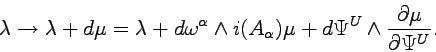
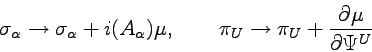
As a further application of the double forms, we consider the addition to the Lagrangian form of an exact term of the kind $d \mu$ , where the 3-form $\mu$ depends only on $\omega^{\alpha}$ and $\Psi^U$, namely on the ``Lagrangian coordinates'', but not on the ``velocities''. We know that the field equations remain unchanged. We have

$$\lambda \to \lambda + d \mu = \lambda + d \omega^{\alpha} \w... ...) \mu + d \Psi^U \wedge \frac{\partial \mu}{\partial \Psi^U}.$$ (4.94)

It follows that

$$\sigma_{\alpha} \to \sigma_{\alpha} + i(A_{\alpha}) \mu, \qquad \pi_U \to \pi_U + \frac{\partial \mu}{\partial \Psi^U}$$ (4.95)

and

$$\theta \to \theta + \hat d \omega^{\alpha} \wedge i(A_{\alph... ...tial \Psi^U} = \theta + \hat d \mu, \qquad \Omega \to \Omega.$$ (4.96)

The symplectic double form $\Omega$ is not affected by the new term.

If the vector field $X$ defined on $\Gamma$ generated a symmetry transformation leaving the Lagrangian invariant, for the corresponding conserved quantity $\theta$ we have

$$\theta = \hat i(X) \theta \to \theta + \hat i(X) \hat d\mu = \theta + X \mu.$$ (4.97)

We see that $\theta$ remains unchanged if $\mu$ is symmetric.