Parallel transport

A fundamental concept in Riemannian geometry is the parallel transport. If a tetrad vector $e_j$ is parallel transported from a point with coordinates $x^{\lambda}$ to a point with coordinates $x^{\lambda} + d x^{\lambda}$, we have (as for any other contravariant four-vector field) [28,30,31,32]

$$\delta e^{\mu}_j = - \Gamma^{\mu}_{\nu \lambda} e^{\nu}_j dx^{\lambda},$$ (1.29)

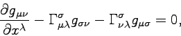
where $\Gamma^{\mu}_{\nu \lambda}$ are the connection coefficients. They depend only on $x^{\lambda}$ and satisfy the metricity condition

$$\frac{\partial g_{\mu \nu}}{\partial x^{\lambda}} - \Gamma^... ...igma \nu} - \Gamma^{\sigma}_{\nu \lambda} g_{\mu \sigma} = 0,$$ (1.30)

that assures that the covariant derivative of the metric tensor vanishes. In a torsionless theory, the connection coefficients are given by the Christoffel symbols.

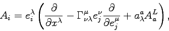
If $n > 0$, the action of a parallel displacement on the group element $g$ is an infinitesimal left translation that depends linearly on $d x^{\lambda}$. In conclusion, a parallel displacement of the tetrads in the direction of the tetrad four-vector $e_i$ is described by the vector field

$$A_i = e^{\lambda}_i \left(\frac{\partial}{\partial x^{\lambd... ...{\partial}{\partial e^{\mu}_j} + a^a_{\lambda} A^L_a \right),$$ (1.31)

where $a^a_{\lambda}(x)$ are the potentials of the gauge field and $A^L_a$ are the generators of the left translations introduced in Section 1.4. In this case too, since we are not dealing with independent variables, we have to verify that the fields (1.31) are tangent to the manifold defined by eq. (1.1), namely that

$$A_i (g_{\mu \nu} e^{\mu}_k e^{\nu}_j) = 0.$$ (1.32)

This is a consequence of the condition (1.30).

After some calculations, we find for the commutators the following expressions

$$[A_{[ik]}, A_j] = \hat F_{[ik]j}^l A_l,$$ (1.33)

$$[A_a, A_j]= 0,$$ (1.34)

$$[A_i, A_k]= 2^{-1} F_{ik}^{[jl]} A_{[jl]} + F_{ik}^j A_j + F_{ik}^a A_a,$$ (1.35)

where

$$\hat F_{[ik]j}^l = g_{kj} \delta_i^l - g_{ij} \delta_k^l,$$ (1.36)

$$F_{ik}^{[jl]} = - e_i^{\lambda} e_k^{\sigma} e^{j}_{\mu} e^{... ...tau} - \Gamma_{\tau \sigma}^{\mu} \Gamma_{\nu \lambda}^{\tau},$$ (1.37)

$$F_{ik}^j = e_i^{\lambda} e_k^{\sigma} e^j_{\mu} S_{\lambda \... ...\Gamma_{\lambda \sigma}^{\mu} - \Gamma_{\sigma \lambda}^{\mu},$$ (1.38)

$$F_{ik}^a = e_i^{\lambda} e_k^{\sigma} D^a{}_d(g^{-1}) F^d_{\... ...rtial x^{\sigma}} - \hat F_{bc}^d a^b_{\lambda} a^c_{\sigma}.$$ (1.39)

The quantities $R^{\mu}_{\nu \lambda \sigma}$, $S_{\lambda \sigma}^{\mu}$ and $F^d_{\lambda \sigma}$ are, respectively, the holonomic components of the Riemann curvature tensor, the torsion tensor and the gauge field strength. The quantities $F_{ik}^{[jl]}$, $F_{ik}^j$ and $F_{ik}^a$ are, up to a sign convention, the anholonomic components of the same tensors, given as functions on $\mathcal{S}_n$.

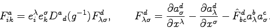
The structure constants (1.36) can be used to write the Lorentz transformation properties of contravariant and covariant four-vectors in the form

$$A_{[ik]} V^j = - \hat F_{[ik]l}^j V^l, \qquad A_{[ik]} V_j = \hat F_{[ik]j}^l V_l.$$ (1.40)