As the theories of gravitation, also the gauge field theories with internal gauge group ![]() [41] have an elegant geometric treatment in the framework of a principal fibre bundle with structural group
[41] have an elegant geometric treatment in the framework of a principal fibre bundle with structural group ![]() [42]. We always specify ``internal'' because gravitation too is described by a gauge theory. If
[42]. We always specify ``internal'' because gravitation too is described by a gauge theory. If
![]() , we obtain Maxwell's electromagnetism and for
, we obtain Maxwell's electromagnetism and for
![]() we have the original Yang-Mills theory [43].
we have the original Yang-Mills theory [43].
Several authors [44,45,46] have proposed a unified treatment of gravitation and internal gauge theories based on a principal fibre bundle with base ![]() and structural group
and structural group
![]() . If
. If ![]() is a Lie group with dimension
is a Lie group with dimension ![]() , this bundle has dimension
, this bundle has dimension ![]() . We call it the bundle of extended frames and we indicate it by
. We call it the bundle of extended frames and we indicate it by ![]() . It can also be considered as a principal fibre bundle with base
. It can also be considered as a principal fibre bundle with base ![]() and structural group
and structural group ![]() . Of course, if
. Of course, if ![]() we have
we have
![]() . This approach is similar to the Kaluza-Klein unification of gravitation and electromagnetism [47,48], but it is conceptually rather different.
. This approach is similar to the Kaluza-Klein unification of gravitation and electromagnetism [47,48], but it is conceptually rather different.
The right action of ![]() on
on ![]() is generated by
is generated by ![]() vector fields
vector fields ![]() , where the index
, where the index ![]() labels a basis of the Lie algebra of
labels a basis of the Lie algebra of ![]() . In the treatment of the Maxwell field, we have
. In the treatment of the Maxwell field, we have ![]() and we indicate the generator of the electromagnetic gauge transformations by
and we indicate the generator of the electromagnetic gauge transformations by ![]() . If
. If ![]() , the vector fields
, the vector fields ![]() satisfy the commutation relations (or Lie brackets)
satisfy the commutation relations (or Lie brackets)
In order to obtain a local parametrization of ![]() , we have to choose, besides a local coordinate system in
, we have to choose, besides a local coordinate system in ![]() , a gauge at every point
, a gauge at every point
![]() . Then the extended frame
. Then the extended frame
![]() is determined by the quantities
is determined by the quantities
![]() , where
, where
![]() , represents the gauge transformation from the conventionally chosen gauge at
, represents the gauge transformation from the conventionally chosen gauge at ![]() to the gauge choice at
to the gauge choice at ![]() . The group element
. The group element ![]() , in turn, can be locally parametrized by
, in turn, can be locally parametrized by ![]() real coordinates. Note that
real coordinates. Note that ![]() is not affected by the right action of the Lorentz group
is not affected by the right action of the Lorentz group ![]() . The generators
. The generators ![]() of the internal gauge transformations also describe the infinitesimal right translations of the group
of the internal gauge transformations also describe the infinitesimal right translations of the group ![]() and there is no problem in using the same symbols for the vector fields defined in
and there is no problem in using the same symbols for the vector fields defined in ![]() and in
and in ![]() .
.
In Section 1.5 we need the vector fields ![]() that generate the left translations on the group
that generate the left translations on the group ![]() . They commute with the generators
. They commute with the generators ![]() of the right translations and satisfy the commutation relations
of the right translations and satisfy the commutation relations
| (1.20) |
| (1.21) |
In Section 1.8 we use the left invariant Maurer-Cartan one-forms ![]() on the gauge group
on the gauge group ![]() defined by the formula
defined by the formula
| (1.22) |
| (1.23) |
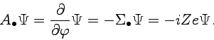
The group ![]() acts linearly on the fields. If, as in eq. (1.14), we consider the field components as the elements of a one-column matrix
acts linearly on the fields. If, as in eq. (1.14), we consider the field components as the elements of a one-column matrix ![]() , we have
, we have
| (1.24) |
| (1.26) |
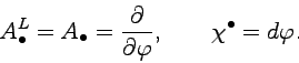
If
![]() ,
, ![]() is a phase factor and it is convenient to put
is a phase factor and it is convenient to put
![]() , where
, where ![]() is a cyclic real parameter with period
is a cyclic real parameter with period ![]() and
and ![]() is the elementary electric charge. In this case we have
is the elementary electric charge. In this case we have
 |
(1.27) |