From these rather boring calculations we have learned several important lessons. We have shown that some scalar fields, which play a peculiar role in modern physics [106], can be generated in a purely geometric way.
We have also seen that we have to carefully choose the Lagrangian in order to get a consistent set of field equations that have a reasonably wide set of solutions. In fact, since the action principle (4.15) must be satisfied for an arbitrary choice of the integration surface ![]() , one often obtains a too restrictive set of field equations. For instance, the choice of the matter Lagrangian is not independent of the choice of the geometric Lagrangian, since eq. (5.45) is necessary in order to avoid a contradiction between the normal equation (6.14) and the tangential equation (6.16)
, one often obtains a too restrictive set of field equations. For instance, the choice of the matter Lagrangian is not independent of the choice of the geometric Lagrangian, since eq. (5.45) is necessary in order to avoid a contradiction between the normal equation (6.14) and the tangential equation (6.16)
Moreover, the functions
![]() cannot be chosen at will, but they must satify eqs. (6.11), (6.17) and (6.19), which are not field equations, but just limitations to the form of the Lagrangian. According to these conditions, that are not independent,
cannot be chosen at will, but they must satify eqs. (6.11), (6.17) and (6.19), which are not field equations, but just limitations to the form of the Lagrangian. According to these conditions, that are not independent, ![]() ,
, ![]() and
and ![]() can be chosen as arbitrary functions of
can be chosen as arbitrary functions of ![]() , but
, but ![]() is uniquely determined and
is uniquely determined and ![]() ,
, ![]() are determined up to an irrelevant additive constant, that adds to the Lagrangian an exact differential form.
are determined up to an irrelevant additive constant, that adds to the Lagrangian an exact differential form.
We are interested in gravitational theories that do not contain the gravitational constant ![]() of Einstein's theory and we also require that they do not contain any other constant with nontrivial dimension (besides the velocity of light). Then
of Einstein's theory and we also require that they do not contain any other constant with nontrivial dimension (besides the velocity of light). Then ![]() has to be a power of
has to be a power of ![]() and a possible numeric constant factor can be absorbed in the definition of the forms
and a possible numeric constant factor can be absorbed in the definition of the forms ![]() . Taking into account the above mentioned constraints, we put, as in ref. [5],
. Taking into account the above mentioned constraints, we put, as in ref. [5],
| (6.26) |
Other interesting results follow from a dimensional analysis. We indicate by ![]() the dimension of time and lenght and by
the dimension of time and lenght and by ![]() the dimension of mass, energy and momentum. Since the coordinates of the manifold
the dimension of mass, energy and momentum. Since the coordinates of the manifold ![]() are dimensionless, the Lagrangian form has the dimension of an action. We have the dimensional relations
are dimensionless, the Lagrangian form has the dimension of an action. We have the dimensional relations
| (6.27) |
| (6.28) |
From eqs. (5.2) and (6.3) we also have
| (6.29) |
In order to write the field equations in a more familiar form, it is convenient to introduce the new vector fields
We also define the new differential 1-forms
![$\textstyle \tilde F_{[ik]j}^i = \phi^{-1} F_{[ik]j}^i = \hat F_{[ik]j}^i, \qqua...
...F_{[ik][jl]}^{[mn]} = \phi^{-1} F_{[ik][jl]}^{[mn]} = \hat F_{[ik][jl]}^{[mn]},$](img1112.png) |
|||
![$\textstyle \tilde F_{[ik][jl]}^m = 0, \qquad
\tilde F_{j[ik]}^{[mn]} = F_{j[ik]}^{[mn]}
- \phi^{-1} A_j \phi (\delta^m_i \delta^n_k - \delta^n_i \delta^m_k) = 0.$](img1113.png) |
|||
![$\textstyle \tilde F_{ik}^j = F_{ik}^j, \qquad \tilde F_{ik}^{[mn]} = \phi F_{ik}^{[mn]}.$](img1114.png) |
(6.33) |
We remark that, after the substitution (6.31), the field ![]() disappears from the Fermion Lagrangian (5.36) and we obtain a theory with a minimal coupling of the kind considered in Section 4.4. We also introduce the quantities
disappears from the Fermion Lagrangian (5.36) and we obtain a theory with a minimal coupling of the kind considered in Section 4.4. We also introduce the quantities
| (6.34) |
Expressed in terms of the new variables, the eqs. (6.13), (6.16), (6.21), take the form
Note that the dependence of the various coefficients on ![]() and in particular the exponent
and in particular the exponent ![]() have disappeared from these equations. This means that the choice of the fundamental fields
have disappeared from these equations. This means that the choice of the fundamental fields ![]() is ambiguous in this macroscopic context, as we discuss in the next Section 6.3.
is ambiguous in this macroscopic context, as we discuss in the next Section 6.3.
If we consider only Dirac spinning particles, from eq. (5.42) we see that eq. (6.36) is equivalent to the equations
We see from eq. (6.35) that, even in the absence of spinning particles, the torsion may not vanish. Since it does not appear in the Brans-Dicke equations, in order to compare them with our formulas, we have to eliminate torsion by changing again the choice of the fundamental vector fields, namely by introducing a torsionless connection, by means of the substitution
| (6.43) |
| (6.44) |
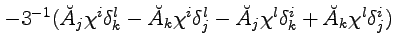
By computing the Lie brackets of the new fields and using eq. (6.39) with ![]() , we obtain the new structure coefficients
, we obtain the new structure coefficients
| (6.45) |
![$\textstyle \breve F_{jk}^{[il]} = \tilde F_{jk}^{[il]}
- 3^{-2} \chi_m \chi^m (\delta_j^i \delta_k^l - \delta_k^i \delta_j^l)$](img1135.png) |
|||
 |
|||
| (6.46) |
By means of these formulas and of eq. (6.41), we can write eqs. (6.35) and (6.37) in the form
The elimination of torsion by means of a different choice of the fundamental vector fields (namely of the connection) is not completely harmless, since the motion of spinning test particles may be influenced by torsion [37].
A comparison with astronomical measurements in the solar systems gives a rather high lower bound on the dimensionless parameter ![]() . Recent data from Cassini-Huygens spacecraft give
. Recent data from Cassini-Huygens spacecraft give
![]() [109]. This means that
[109]. This means that
![]() and the field
and the field ![]() is approximately constant. Then the limit
is approximately constant. Then the limit
![]() or
or
![]() of the Brans-Dicke equations is physically very interesting, but it is not trivial [110].
of the Brans-Dicke equations is physically very interesting, but it is not trivial [110].
In our geometric approach, however, we can introduce the choice ![]() from the begining directly in eq. (6.30), in the Lagrangian (6.3) and in eqs. (6.35), (6.37) and (6.39). From eq. (6.40) we see that
from the begining directly in eq. (6.30), in the Lagrangian (6.3) and in eqs. (6.35), (6.37) and (6.39). From eq. (6.40) we see that ![]() , namely
, namely
![]() is constant. From eq. (6.20) and (6.2) we also obtain
is constant. From eq. (6.20) and (6.2) we also obtain
| (6.50) |
In this way, we obtain a theory with a constant gravitational coupling, that is not determined by the theory, but by the initial conditions. It also has a dynamical torsion, since the quantities ![]() , that represent the 4-vector part of the torsion, are true dynamical variables and their derivatives appear in the field equations. Theories with a dynamical torsion have been proposed by various authors.
, that represent the 4-vector part of the torsion, are true dynamical variables and their derivatives appear in the field equations. Theories with a dynamical torsion have been proposed by various authors.
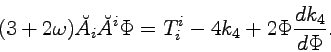
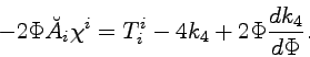
If the spin density vanishes, by introducing the new fields
![]() , we obtain the equations
, we obtain the equations
| (6.51) |
 |
(6.52) |
 before performing the limit
The first formula is just the field equation of general relativity. The second formula determines only partially the vector field ![]() that, since torsion has been eliminated, has lost its geometric meaning and does not give any contribution to the source of the gravitational field. These properties of
that, since torsion has been eliminated, has lost its geometric meaning and does not give any contribution to the source of the gravitational field. These properties of ![]() are hardly acceptable from the physical point of view. One may suggest that the model in not complete and that new terms have to be added to the Lagrangian. We shall consider again this suggestion in Chapter 7.
are hardly acceptable from the physical point of view. One may suggest that the model in not complete and that new terms have to be added to the Lagrangian. We shall consider again this suggestion in Chapter 7.
![\begin{displaymath}
2^{-1} \tilde F_{ik}^{[ik]} + \frac{d k_4}{d \Phi} - \alpha \chi_i \chi^i = 0,
\end{displaymath}](img1118.png)
![$\textstyle \Phi (- \tilde F_{jk}^{[ik]} + 2^{-1} \delta^i_j \tilde F_{lk}^{[lk]})
+ 2 \alpha (\chi^i A_j \Phi - \chi^k A_k \Phi \delta^i_j)$](img1120.png)
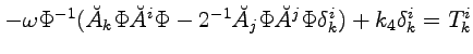
![\begin{displaymath}
- \breve F_{ik}^{[ik]} + 2 \omega \Phi^{-1} \breve A_j \brev...
... \breve A_j \Phi \breve A^j \Phi
- 2 \frac{d k_4}{d \Phi} = 0,
\end{displaymath}](img1138.png)
![$\textstyle \Phi (- \breve F_{kj}^{[ij]} + 2^{-1} \breve F_{jl}^{[jl]} \delta^i_k)
- \breve A_k \breve A^i \Phi
+ \breve A_j \breve A^j \Phi \delta^i_k$](img1139.png)