A very interesting class of generalizations of Einstein's theory is based on the replacement of the gravitational constant ![]() by a variable scalar field [69,70,71]. A motivation for this assumption is the explanation of the extremely small value of
by a variable scalar field [69,70,71]. A motivation for this assumption is the explanation of the extremely small value of ![]() when measured in atomic units (Dirac's large numbers problem). According to these theories, the value of the scalar field that replaces
when measured in atomic units (Dirac's large numbers problem). According to these theories, the value of the scalar field that replaces ![]() is determined by the distribution of matter in the universe, in agreement with the ideas of Mach [103] on the influence of very far celestial bodies on the locally observed phenomena. The best known Lagrangian scalar-tensor theory of this kind has been proposed by Brans and Dicke [71] and theories including torsion have been discussed in ref. [104].
is determined by the distribution of matter in the universe, in agreement with the ideas of Mach [103] on the influence of very far celestial bodies on the locally observed phenomena. The best known Lagrangian scalar-tensor theory of this kind has been proposed by Brans and Dicke [71] and theories including torsion have been discussed in ref. [104].
We think that it is important to give to this scalar field a geometric interpretation, by writing it as a function of the structure coefficients, in agreement with the idea that all the structure coefficients should have a dynamical relevance. In the discussion of this problem we also clarify some concepts introduced in Chapters 2 and 3 and we introduce some ideas useful for the developments of Chapter 7.
We have seen in Section 5.2 that one can include the coupling constants of a Yang-Mills theory in the structure constants ![]() of the gauge group. If the coupling constant becomes a variable [105], these structure coefficients acquire a dynamical role. In a similar way, one can try to include the gravitational constant
of the gauge group. If the coupling constant becomes a variable [105], these structure coefficients acquire a dynamical role. In a similar way, one can try to include the gravitational constant ![]() , or the variable field that replaces it, in the structure constants
, or the variable field that replaces it, in the structure constants
![$F_{[ik][jl]}^{[mn]}$](img1051.png) and
and ![]() of the Poincaré group. A theory of this kind, equivalent, if spin is neglected, to the Brans-Dicke theory [71], has been discussed in ref. [5]. Here we give a slightly different treatment.
of the Poincaré group. A theory of this kind, equivalent, if spin is neglected, to the Brans-Dicke theory [71], has been discussed in ref. [5]. Here we give a slightly different treatment.
We define the scalar field ![]() by means of the formula
by means of the formula
![$F_{[ik]j}^i = \hat F_{[ik]j}^i$](img1054.png) , we obtain
, we obtain
Moreover, we have to add new terms to the Lagrangian, in order to obtain the field equations that determine the field ![]() starting from the matter distribution in the universe and from suitable initial conditions. It seems that these new terms should contain the derivatives
starting from the matter distribution in the universe and from suitable initial conditions. It seems that these new terms should contain the derivatives ![]() , but we want to avoid the appearance in the Lagrangian of derivatives of the structure coefficients. We try to use for the same purpose suitable functions of the structure coefficients, increasing in this way their physical role, in agreement with our program.
, but we want to avoid the appearance in the Lagrangian of derivatives of the structure coefficients. We try to use for the same purpose suitable functions of the structure coefficients, increasing in this way their physical role, in agreement with our program.
The structure coefficients that appear in the forms
![]() are not sufficient and we have to introduce some other expressions
are not sufficient and we have to introduce some other expressions ![]() . After several attempts, one finds that it is convenient to put
. After several attempts, one finds that it is convenient to put
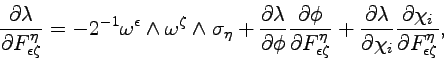
The derivatives of ![]() that appear in the normal field equation (4.28) contain two contributions, one coming from the forms
that appear in the normal field equation (4.28) contain two contributions, one coming from the forms
![]() and the other originated by the dependence on the quantities
and the other originated by the dependence on the quantities ![]() and
and ![]() , namely we have
, namely we have
 |
(6.4) |
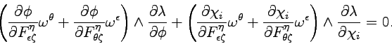
The first contribution satisfies the normal field equation automatically and the second contribution gives the condition
 |
(6.6) |
![\begin{displaymath}
\omega^{[jk]} \wedge \frac{\partial \lambda}{\partial \phi} ...
...ga^{[jk]} \wedge \frac{\partial \lambda}{\partial \chi_i} = 0.
\end{displaymath}](img1066.png) |
(6.7) |
For a given value of ![]() , the condition
, the condition
![]() implies that the form
implies that the form ![]() is proportional to
is proportional to ![]() . If we require that this condition holds for all the six values of
. If we require that this condition holds for all the six values of ![]() , either
, either ![]() vanishes or it is a form of degree not smaller than 6. In conclusion, we obtain the conditions
vanishes or it is a form of degree not smaller than 6. In conclusion, we obtain the conditions
We assume that ![]() does not depend on
does not depend on ![]() and that its dependence on
and that its dependence on ![]() is given by eq. (5.45). The normal equation (6.9) involves only the additional Lagrangian
is given by eq. (5.45). The normal equation (6.9) involves only the additional Lagrangian
![]() and it is equivalent to the conditions
and it is equivalent to the conditions
In order to obtain simpler and more consistent results, we choose the functions ![]() ,
, ![]() and
and ![]() in such a way that
in such a way that
From eqs. (6.10) and (6.12) and the special case
![]() of the generalized Jacobi identity (1.55), we see that
of the generalized Jacobi identity (1.55), we see that
The eqs. (5.5), (5.6) and (5.7) are still valid and the explicit equations (5.8) and (5.9) contain additional terms proportional to ![]() and to the derivatives of
and to the derivatives of ![]() and
and ![]() . By performing the calculations, if the 10-momentum of matter has the local form (4.68), from the vertical tangential equation we obtain first of all the condition
. By performing the calculations, if the 10-momentum of matter has the local form (4.68), from the vertical tangential equation we obtain first of all the condition
Continuing the analysis of the vertical tangential equation, we see that it is compatible with eq. (6.10) only if we choose
By using the conditions (6.10), from the generalized Jacobi identity (1.55) we obtain the formula
| (6.22) |
| (6.23) |
Note that, if we put ![]() from eqs. (6.13) and (6.21) we have the condition
from eqs. (6.13) and (6.21) we have the condition
| (6.24) |
Attempts to generalize the above discussed model by introducing anisotropic features of the gravitational field are discussed in ref. [108].


![$\textstyle 4 k (- F_{jk}^{[ik]} + 2^{-1} \delta^i_j F_{lk}^{[lk]})
- 2 k'_5 (\chi^i A_j \phi - \chi^k A_k \phi \delta^i_j)$](img1090.png)