Internal gauge theories

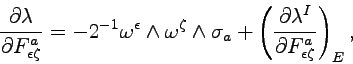
A Lagrangian form in an extended space $\mathcal{S}$ describing Maxwell's electromagnetism has been proposed in ref. [3] and it has been generalized to noncommutative gauge theories in ref. [54]. In order to give a motivation, in the electromagnetic case one can start from the Maxwell form $\sigma_{\bullet}$ defined in eq. (4.12), which appears in the Gauss law (4.13). The generalization to an arbitrary internal gauge theory is

$$\sigma_a = 2^{-2} G_{ab} F^b_{ik} \epsilon^{ik}{}_{jl} \, \omega^j \wedge \omega^l, \qquad d \sigma_a = - \tau_a,$$ (5.12)

where the nondegenerate real symmetric matrix $G_{ab}$ is invariant under the internal gauge group $\mathcal{G}$, namely it has the property

$$\hat F^d_{ab} G_{dc} + \hat F^d_{ac} G_{bd} = 0.$$ (5.13)

Eq. (5.12) can be obtained from the extended geometric Lagrangian form $\lambda^G = \lambda^H + \lambda^A + \lambda^I$ where the new term is given by

$$\lambda^I= d \omega^a \wedge \sigma_a + 2^{-3} G_{ab} \hat F^a_{cd} ... ...epsilon^{ik}{}_{jl} \, \omega^c \wedge \omega^d \wedge \omega^j \wedge \omega^l$$

$$+ 2^{-2} G_{ab} F^a_{ik} F^b_{jl} g^{ij} g^{kl} \eta.$$ (5.14)

In the usual formulation of the Standard Model of the elementary particles, the matrix $G_{ab}$ contains the coupling constants of the theory. Alternatively, one can rescale the vector fields $A_a$ the forms $\omega^a$, the structure constants $\hat F^a_{bc}$ and the matrices $\Sigma_a$ in such a way that $G_{ab} = \delta_{ab}$. Then, the coupling constants are contained in $\hat F^a_{bc}$ and in $\Sigma_a$. For the Maxwell theory we adopt the standard convention with rationalized units, namely we put $G_{\bullet\bullet} = 1$ and the coupling constant, namely the elementary charge, appears in $\Sigma_{\bullet}$, namely in the gauge transformation law of the charged fields given by eq. (1.28). If one prefers nonrationalized units, one has to put $G_{\bullet\bullet} = (4 \pi)^{-1}$.

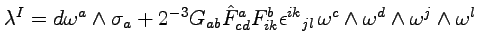
The Lagrangian form (5.14) depends only on the structure coefficients $F^a_{\alpha \beta}$ with $a \geq 10$, while these coefficients do not appear in the other parts of the Lagrangian form $\lambda$. The partial derivatives of $\lambda$ with respect to $F^a_{\alpha \beta}$ have a contribution from the structure coefficients implicitly contained in $d \omega^a$ and a contribution from the structure coefficients explicitly present in the Lagrangian, namely we have

$$\frac{\partial \lambda}{\partial F_{\epsilon \zeta}^a} = - ... ...c{\partial \lambda^I}{\partial F_{\epsilon \zeta}^a}\right)_E,$$ (5.15)

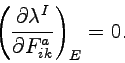
where the subscript $E$ indicates the second contribution, that, as we see from eq. (5.14), vanishes if $\epsilon > 3$ or $\zeta > 3$. The first contribution disappears from the normal field equation (4.28) and we easily see that, for $\eta = a$, this equation is equivalent to the simpler condition

$$\left(\frac{\partial \lambda^I}{\partial F_{ik}^a}\right)_E =0.$$ (5.16)

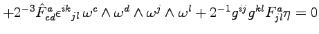
More explicitly we have

$$- 2^{-3} F^a_{\alpha \beta} \epsilon^{ik}{}_{jl} \, \omega^{\alpha} \wedge \omega^{\beta} \wedge \omega^j \wedge \omega^l$$

$$+ 2^{-3} \hat F^a_{cd} \epsilon^{ik}{}_{jl} \, \omega^c \wedge \omega^d \wedge \omega^j \wedge \omega^l + 2^{-1} g^{ij} g^{kl} F^a_{jl} \eta = 0$$ (5.17)

and, considering various values of the indices $\alpha$ and $\beta$, we obtain the normal field equations in the form

$$F^a_{bc} = \hat F^a_{bc}, \qquad F^a_{\beta \gamma} = - F^a_{\gamma \beta} = 0, \quad \beta \leq 9, \quad \alpha \geq 4.$$ (5.18)

If these equations are satisfied, the quantity (5.12) is the same that appears in eq. (4.31) and we have

$$\lambda^I = - 2^{-2} G_{ab} F^a_{ik} F^b_{jl} g^{ij} g^{kl} \eta.$$ (5.19)

We describe gravitation as in Section 5.1, but in the extended space $\mathcal{S}$. The presence of $\lambda^I$ affects the tangential field equations (4.59) by adding to the source term $\tau^M_i$ the new term

$$\tau^I_i = F_{ik}^a \, \omega^k \wedge \sigma_a + i_i \lambda^I = I^j_i \eta_j,$$

$$I^j_i = G_{ab} (F^a_{im} F^b_{ln} g^{mn} g^{lj} - 2^{-2} F^a_{pm} F^b_{qn} g^{mn} g^{pq} \delta^j_i),$$ (5.20)

that represents the energy-momentum of the gauge field. There is no contribution of the gauge field to the spin density, in agreement with the treatment given in ref. [37]. The energy density cannot be negative, namely

$$I^{00} = - I^0_0 = 2^{-1} G_{ab} F^a_{0r} F^b_{0s} g^{rs} \geq 0,$$ (5.21)

if the matrix $G_{ab}$ is positive definite.

There also is the additional tangential field equation

$$d \sigma_a + \hat F_{ab}^c \, \omega^b \wedge \sigma_c = - \tau^M_a,$$ (5.22)

where the right hand side describes the charges of matter. The second term in the left hand side, that describes the charges of the Yang-Mills field, is absent in Maxwell's theory. Note that it is not spatially localized, since it contains $\omega^b$.

If $\tau^M_a$ is spatially localized, eq. (5.22) can be written in the more explicit form

$$G_{ab} (g^{ij} g^{kl} A_l F^b_{ik} - g^{ij} g^{kl} F^m_{lm} F^b_{ik} - 2^{-1} g^{im} g^{kn} F^j_{mn} F^b_{ik}) = - T_a^j,$$ (5.23)

$$A_a F^b_{ik} = - \hat F^b_{ac} F^c_{ik}, \qquad A_{[ik]} F^a_{jl} = \hat F^m_{[ik]j} F^a_{ml} + \hat F^m_{[ik]l} F^a_{jm}.$$ (5.24)

The first formula is the Yang-Mills field equation with torsion corrections. In particular it gives the inhomogeneous Maxwell equations. The other formulas give the transformation properties of the gauge field strength with respect to gauge and Lorentz transformations. As we have observed in Section 1.7, these properties also follow from eq. (1.55). From the same general formula we also obtain the equation

$$A_i F^a_{jk} + A_j F^a_{ki} + A_k F^a_{ij} - F^l_{ij} F^a_{lk} - F^l_{jk} F^a_{li} - F^l_{ki} F^a_{lj} = 0,$$ (5.25)

that in the electromagnetic theory is just the homogeneous Maxwell equation.

Note that, in this case too, the typical properties of the structure coefficients of a principal fibre bundle are consequences of the action principle.