The Lagrangians studied in Chapter 5 have a particular structure that permits a simpler treatment of the normal field equations. In the present Chapter too, we consider Lagrangian of the form
The derivatives of ![]() with respect to the structure coefficients that appear in the normal field equation (4.28) contain two contributions, one coming from the exterior derivatives
with respect to the structure coefficients that appear in the normal field equation (4.28) contain two contributions, one coming from the exterior derivatives
![]() and the other originated by the dependence of
and the other originated by the dependence of ![]() on the quantities
on the quantities ![]() and
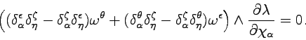
and ![]() . The first contribution satisfies the normal field equations automatically and the second contribution gives the condition
. The first contribution satisfies the normal field equations automatically and the second contribution gives the condition
| (7.21) |
We fix arbitrarily the indices ![]() and
and ![]() , and without loss of generality we assume, for instance, that
, and without loss of generality we assume, for instance, that ![]() . Then we chose
. Then we chose
![]() and
and
![]() . We choose the other indices
. We choose the other indices ![]() in such a way that
in such a way that
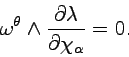
![]() are all different. Then only the first term of eq. (7.20) survives and we have
are all different. Then only the first term of eq. (7.20) survives and we have
![\begin{displaymath}
\omega^{[xx'5]} \wedge \frac{\partial \lambda}{\partial f_u} = 0.
\end{displaymath}](img1246.png) |
(7.22) |
In order to treat the second part of eq. (7.19), we write it in the form
 |
(7.24) |
 |
(7.25) |
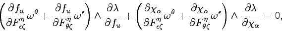
For the particular kind of Lagrangians we are considering, eqs. (7.23) and (7.26) are equivalent to the normal equation (4.28). By introducing the variables ![]() , eq (7.23) can also be written in the form
, eq (7.23) can also be written in the form
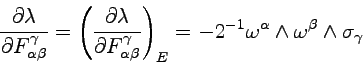
From eq. (7.17) and the normal field equations (7.23) and (7.26) we have
The conservation laws corresponding to the infinitesimal
![]() symmetry transformations play an important role in the following discussion. As it is explained in Section 4.5, these transformations are generated by the vector fields
symmetry transformations play an important role in the following discussion. As it is explained in Section 4.5, these transformations are generated by the vector fields ![]() (in the phase space) that act on the dynamical variables in the following way
(in the phase space) that act on the dynamical variables in the following way
According to eq. (4.41), this symmetry gives rise to the conservation laws
These conservation laws, are a consequence of all the field equations and we want to show that, when all the other field equations are satisfied, the normal equation (7.27) is equivalent to the following equation that sometimes has an easier treatment and a more direct meaning:
We use the invariance property of ![]() , which, using the shorthand notation introduced in Section 7.1, can be written in the form
, which, using the shorthand notation introduced in Section 7.1, can be written in the form
![\begin{displaymath}
X_{[uv]} \lambda = X_{[uv]} Z \frac{\partial \lambda}{\parti...
...+ X_{[uv]} \psi_w \frac{\partial \lambda}{\partial \psi_w}= 0,
\end{displaymath}](img1264.png) |
(7.34) |
| (7.35) |
By means of the normal field equation (4.29) and of the tangential equations (4.34), (4.35) and (4.36), we obtain
| (7.36) |
![\begin{displaymath}
d \theta_{[uv]} + (g_{uw} \psi_v - g_{vw} \psi_u) \frac{\partial \lambda}{\partial \psi_w} = 0.
\end{displaymath}](img1271.png) |
(7.37) |
If the normal equation (7.27) is satisfied (as well as all the other field equations) this is just a new proof of the conservation of ![]() . Conversely, if we assume eq. (7.33), we easily obtain the normal equation (7.27), as we have anticipated above.
. Conversely, if we assume eq. (7.33), we easily obtain the normal equation (7.27), as we have anticipated above.
In the analysis of the field equations, a considerable simplification can be obtained by choosing an adapted basis in the space ![]() by means of a suitable (global) transformation of the symmetry group
by means of a suitable (global) transformation of the symmetry group
![]() . In this way, assuming the inequality (7.8), we can put, at a single distinguished point
. In this way, assuming the inequality (7.8), we can put, at a single distinguished point
![]() ,
, ![]() or
or ![]() . At this point the Lagrangian form
. At this point the Lagrangian form ![]() is not affected by the substitution rule. Besides
is not affected by the substitution rule. Besides ![]() , also
, also ![]() ,
,
![]() ,
, ![]() , and
, and ![]() have, at the particular point
have, at the particular point ![]() , the same form they have before the application of the substitution rule. In particular, the quantities
, the same form they have before the application of the substitution rule. In particular, the quantities
![]() have the local form (4.68).
have the local form (4.68).
However, one has to be careful in dealing with expressions containing derivatives with respect to ![]() or other differential operators applied to expressions containing
or other differential operators applied to expressions containing ![]() : one has to compute the derivatives first and then to put
: one has to compute the derivatives first and then to put ![]() . For instance, the field equations and the conservation laws may contain new terms that do not vanish at the point
. For instance, the field equations and the conservation laws may contain new terms that do not vanish at the point ![]() . In order to compute them, we need the derivatives of various quantities with respect to
. In order to compute them, we need the derivatives of various quantities with respect to ![]() at the point
at the point ![]() .
.
In some simple cases, these derivatives can be obtained directly or by means of eq. (7.16). They can also be obtained by means of the covariance of these quantities with respect to the infinitesimal transformations ![]() given by
given by
| (7.38) |
| (7.39) |
By using the shorthand notation introduced at the end of Section 7.1, since at the point ![]() it is
it is
| (7.40) |
In many situations the ``old'' theory, considered before the application of the substitution rule, agrees with a good accuracy with the empirical data. As a consequence, it is important to understand the conditions under which the solutions of the ``old'' theory are also solutions of the ``new'' theory obtained by means of the substitution rule. For these solutions we have
 and the corrections to the field equations, proportional to derivatives of
 ![]() vanish. However, the ``new'' theory has the additional normal equation (7.27), equivalent to the conservation law (7.33), that in the case we are considering takes the form
vanish. However, the ``new'' theory has the additional normal equation (7.27), equivalent to the conservation law (7.33), that in the case we are considering takes the form
![]() . If and only if it astisfies this equation a solution of the ``old'' theory is also a solution of the ``new'' theory.
. If and only if it astisfies this equation a solution of the ``old'' theory is also a solution of the ``new'' theory.
![$\textstyle \alpha \left((\delta_u^v \epsilon_{yy'}{}^{v'ww'}
- \delta_u^{v'} \e...
...{yy'}{}^{w'vv'}
+ \delta_u^{w'} \epsilon_{yy'}{}^{wvv'}) \omega^{[xx'5]}\right.$](img1234.png)
![$\textstyle \left. + (\delta_u^x \epsilon_{yy'}{}^{x'ww'}
- \delta_u^{x'} \epsil...
...{}^{wxx'}) \omega^{[vv'5]} \right)
\wedge \frac{\partial \lambda}{\partial f_u}$](img1235.png)
![$\textstyle + \beta \left((\delta_{uu'}^{vv'} \delta_{yy'}^{ww'} - \delta_{uu'}^{ww'} \delta_{yy'}^{vv'})
\omega^{[xx'5]}\right.$](img1236.png)
![$\textstyle \left. + (\delta_{uu'}^{xx'} \delta_{yy'}^{ww'} - \delta_{uu'}^{ww'}...
...ga^{[vv'5]} \right)
\wedge \frac{\partial \lambda}{\partial \chi_{[uu'5]}} = 0,$](img1237.png)


![$\textstyle \frac{\partial \sigma_j}{\partial \psi^i}
= - 2^{-1} \ell^{-1} \epsilon_{ji}{}^{kl} \sigma_{[kl]}
- \frac{\partial \sigma_j}{\partial Z} X_{[i4]} Z,$](img1283.png)
![$\textstyle \frac{\partial \sigma_{[jk]}}{\partial \psi^i}
= - \ell \epsilon_{jki}{}^l \sigma_l
- \frac{\partial \sigma_{[jk]}}{\partial Z} X_{[i4]} Z,$](img1284.png)
![$\textstyle \frac{\partial \theta_{[jk]}}{\partial \psi^i} = g_{ik} \theta_{[j4]}
- g_{ij} \theta_{[k4]} - \frac{\partial \theta_{[jk]}}{\partial Z} X_{[i4]} Z,$](img1285.png)
![$\textstyle \frac{\partial \theta_{[j4]}}{\partial \psi^i}
= \theta_{[ji]} - \frac{\partial \theta_{[j4]}}{\partial Z} X_{[i4]} Z.$](img1286.png)